Pressure Drop Calculator
Pressure Drop Calculator
Results
Pressure drop, often denoted as ΔP, is the reduction in fluid pressure as it moves through a system. This phenomenon is not a design flaw but a physical necessity; it represents the energy required to push the fluid through pipes, ducts, fittings, and equipment. Every time a fluid—whether water, air, or oil—interacts with a pipe wall, changes direction, or passes through a valve, it loses a minute amount of its driving energy. This lost energy manifests as a decrease in pressure.
The primary cause of this loss is friction. As a fluid flows, a boundary layer forms along the pipe wall. The roughness of the pipe material creates drag, slowing the fluid molecules immediately adjacent to the surface. This frictional resistance converts kinetic energy into heat, which is effectively lost from the system’s pressure head . Beyond straight pipe friction, other components contribute significantly. Turbulence generated by tees, elbows, and valves, as well as sudden expansions or contractions in the pipe diameter, all consume energy. In systems with elevation changes, the static head—the force required to lift the fluid against gravity—also imposes a pressure demand on the system .
Engineers and builders calculate this loss before installation to ensure a system is both functional and economical. A pipe that is too narrow for a given flow rate will result in excessive velocity and friction, leading to a pressure drop so high that the pump or fan cannot maintain the required flow at the end of the line. Conversely, oversizing pipes minimizes pressure loss but increases material costs unnecessarily . A pressure-drop calculator provides the quantitative analysis needed to strike this balance. It is a fundamental tool in the design of:
- Plumbing systems: To guarantee adequate water pressure at fixtures on upper floors.
- HVAC duct design: To ensure fans can overcome duct friction and deliver design airflow to rooms.
- Industrial piping: For sizing pumps in process plants, refineries, and cooling water systems .
- Irrigation systems: To design zones that operate within available water pressure.
- Fire protection lines: To verify that sprinkler heads receive sufficient pressure and flow as mandated by safety codes .
- Water distribution systems: To model pressure losses in municipal mains.
By predicting system behavior before construction, the calculator prevents costly design errors like pump cavitation, inadequate flow, or the need for oversized motors.
How the Pressure Drop Calculator Works (Conceptual Overview)
The calculator simulates fluid behavior by applying empirical and theoretical relationships between key physical variables. At its core, the calculation logic recognizes that pressure loss is not random but a function of measurable parameters. The fundamental relationship involves the fluid's velocity; higher speeds exponentially increase friction losses. The pipe's internal diameter is equally critical—a small reduction in diameter can drastically increase resistance, as the fluid is forced to interact more intensely with a proportionally larger wall surface. The total length of the pipeline directly compounds this friction, while the fluid's own properties, namely its density and viscosity, dictate how easily it shears and flows. Finally, the internal roughness of the pipe material (e.g., steel versus PVC) determines the level of frictional drag at the wall .
The calculator processes these inputs to solve for pressure loss using established engineering equations. It first determines the flow regime—whether the fluid motion is smooth and orderly (laminar) or chaotic (turbulent)—by calculating the Reynolds Number. This regime then dictates which formula is used to find the friction factor, a dimensionless coefficient that quantifies the resistance of the pipe. This friction factor, combined with the pipe geometry and fluid velocity, yields the final pressure drop value .
Major Causes of Pressure Drop
- Friction Losses (Major Losses): The pressure drop due to the fluid's viscosity and its interaction with the pipe wall over its entire length. This is the dominant loss in long, straight pipe runs .
- Minor Losses: Losses caused by fittings, valves, bends, and changes in cross-section. While termed "minor," they can be the largest losses in a system with many components, such as a pump station or a plant
- Entrance and Exit Losses: The pressure drop as fluid enters a pipe from a large reservoir (due to flow contraction) and exits back into a reservoir (due to sudden expansion).
- Elevation Changes: In liquid systems, pumping fluid uphill requires overcoming the static head, which is a pressure increase required, not a frictional loss. However, it is a net pressure change the calculator must account for [
Pipe Roughness and Material Effects
The interior surface of a pipe is rarely perfectly smooth. The average height of the surface irregularities is termed absolute roughness (ε). This value varies significantly by material:
- Steel pipes: Commercial steel has a moderate roughness that can increase over time with corrosion or scaling.
- Copper pipes: Typically smooth, with low absolute roughness.
- PVC and HDPE: These plastics are hydraulically smooth, offering very low friction compared to metallic pipes.
- Concrete pipes: Used in large-scale civil works, they have a high roughness value due to the surface texture .
Major vs Minor Losses
Major losses are calculated along the pipe's length using the Darcy-Weisbach or Hazen-Williams formulas. Minor losses are typically calculated using the equivalent length method or the K-factor method, where the loss is a multiple of the velocity head .
Reynolds Number and Flow Regime
The Reynolds Number (Re) is a dimensionless value that predicts flow patterns. It is the ratio of inertial forces to viscous forces.
- Laminar flow (Re < 2000): Fluid moves in smooth, parallel layers. Friction is independent of pipe roughness and is solely a function of Re .
- Turbulent flow (Re > 4000): Flow is chaotic with eddies and vortices. Friction depends on both Re and pipe roughness. Most practical construction applications fall into this category .
- Transitional region (2000 < Re < 4000): Flow is unstable and difficult to predict accurately.
Darcy Friction Factor
The friction factor (f or λ) is a variable used in the Darcy-Weisbach equation. For laminar flow, f = 64/Re. For turbulent flow, it is found using the Colebrook-White equation, which requires iteration, or the explicit Swamee-Jain approximation .
Friction Loss Tables
Pre-calculated tables are often used for quick estimates, showing pressure loss per 100 feet (or 100 meters) of pipe for various diameters and flow rates. These are typically derived from the Hazen-Williams formula for water.
Equivalent Length Method
A technique to estimate minor losses by expressing the pressure drop through a fitting as the equivalent length of straight pipe that would cause the same frictional loss. This length is added to the actual pipe length before calculating total loss.
Flow Velocity Considerations
Velocity directly impacts pressure drop (ΔP ∝ v²). Design standards often provide maximum recommended velocities to prevent erosion, water hammer, and high noise levels. For example, typical water velocity in pipes is often kept around 4-8 ft/s (1.2-2.4 m/s).
Pipe Diameter Selection
There is an economic trade-off. Smaller pipes are cheaper to buy but more expensive to operate due to higher pumping costs. Larger pipes have a higher upfront cost but lower energy costs over the system's life.
Temperature and Fluid Property Effects
Temperature changes alter a fluid's density and, more significantly, its viscosity. For example, hot water is less viscous than cold water, which reduces the Reynolds number and affects the friction factor .
Pressure Drop in Duct Systems
For air ducts, the same principles apply, but the calculations often use friction charts or specific equations from ASHRAE. Duct material (galvanized steel, flex duct) has specific roughness values that influence friction .
Pressure Drop in Liquid vs Gas Systems
For liquids, density is typically constant (incompressible flow). For gases, as pressure drops, the gas expands, and velocity increases. This requires more complex calculations for compressible flow, especially at high pressures or velocities (approaching 40% of sonic velocity) .
Static vs Dynamic Pressure
In a fluid, static pressure acts in all directions (the pressure measured by a gauge), while dynamic pressure is associated with the fluid's motion. Pressure drop primarily refers to the irreversible loss of total pressure (static + dynamic).
Head Loss vs Pressure Loss
Head loss (hf) is the height of a fluid column that the lost pressure represents. It is related by ΔP = ρ * g * hf. While pressure loss depends on fluid density, head loss (in meters or feet of fluid) is independent of fluid type, making it useful for pump selection .
Pipe Network Considerations
In complex networks, pressure drops are additive in series. In parallel, flow splits based on the resistance of each branch, analogous to electrical circuits .
Design Safety Margins
Engineers often add a safety factor (e.g., 10-15%) to calculated pressure drops to account for pipe aging, unforeseen fittings, and uncertainties in roughness, ensuring the pump is not undersized .
Mathematical / Formula Explanation
The accuracy of a pressure drop calculator hinges on the underlying fluid mechanics equations. The primary relationships are as follows.
Darcy–Weisbach Equation
This is the most theoretically accurate and widely applicable equation for calculating frictional head (or pressure) loss in a pipe, valid for all flow regimes and fluids .
ΔP = f × (L / D) × (ρ × v² / 2)
Where:
- ΔP = Pressure drop (Pa, psi)
- f = Darcy-Weisbach friction factor (dimensionless)
- L = Length of pipe (m, ft)
- D = Internal pipe diameter (m, ft)
- ρ = Fluid density (kg/m³, lb/ft³)
- v = Average fluid velocity (m/s, ft/s)
The term (ρv²/2) is the dynamic pressure. The equation assumes steady, incompressible flow in a straight, circular pipe with a fully developed velocity profile .
Head Loss Formula
The same equation can be rearranged to give head loss (hf), which is the energy loss expressed as a column height of the flowing fluid.
hf = f × (L / D) × (v² / 2g)
Where g is the acceleration due to gravity (9.81 m/s², 32.2 ft/s²). This form is common in pump and turbine analysis .
Hazen–Williams Formula
An empirical formula used almost exclusively for water in turbulent flow at ordinary temperatures (around 60°F or 15.5°C). It is simpler because it does not require a separate friction factor, but it is less accurate and cannot be used for other fluids or laminar flow.
hf = (10.67 × L × Q^1.852) / (C^1.852 × D^4.87) (for SI units with m, m³/s)
Where C is the Hazen-Williams roughness coefficient (e.g., 150 for PVC, 120 for new steel, 100 for cast iron).
Minor Loss Formula
Losses through fittings are calculated using a loss coefficient (K), which is specific to the fitting geometry and size.
h_minor = K × (v² / 2g)
ΔP_minor = K × (ρ × v² / 2)
K values are empirically determined. For example, a standard 90° elbow might have a K of 0.75, while a fully open gate valve might have a K of 0.2 .
Practical Real-World Examples
Example 1: Residential Plumbing Line
A 50-meter run of 20mm internal diameter (ID) PVC cold water line is designed to carry 0.3 L/s. The system includes 10 standard 90° elbows.
Fluid: Water at 20°C (ρ = 998 kg/m³, μ = 0.001 Pa·s).
Velocity: Calculated from flow and area (approx. 0.95 m/s).
Reynolds Number: ~19,000 (Turbulent).
Major Loss: Using Darcy-Weisbach with a friction factor of ~0.026, the loss is calculated at 15.7 kPa.
Minor Loss: 10 elbows (K=0.9 each) create a loss of 4.1 kPa.
Total Pressure Drop: 19.8 kPa. The designer confirms this is acceptable and the pressure at the farthest tap will be adequate.
Example 2: HVAC Duct System
An air handling unit supplies 1000 L/s (2100 CFM) through a 30-meter-long galvanized steel duct with a diameter of 400 mm.
Fluid: Air at 20°C (ρ = 1.2 kg/m³).
Velocity: 7.96 m/s.
Friction Loss: Using duct friction charts based on the Darcy-Weisbach equation, the loss is approximately 0.8 Pa/m.
Total Pressure Drop: 24 Pa. This value is used to select a fan that can deliver the required airflow against this system resistance.
Example 3: Industrial Long Pipeline
A 2-kilometer section of DN 150 (6-inch) schedule 40 steel pipe transports oil at a rate of 50 L/s. The elevation gain is 15 meters.
Fluid: Oil (ρ = 850 kg/m³, kinematic viscosity = 40 cSt).
Velocity: 2.83 m/s.
Reynolds Number: ~10,600 (Turbulent).
Static Head: The elevation gain requires an additional pressure of ρ*g*h = 125 kPa.
Frictional Loss: Calculated via Darcy-Weisbach with a friction factor of 0.031, the frictional pressure drop is 1100 kPa.
Total Required Pump Discharge Pressure: The sum of static head and frictional loss (1225 kPa). This calculation shows that despite the high friction, the static lift is a smaller component of the total load.
Limitations, Assumptions & Edge Cases
All calculators operate within a set of assumptions, and understanding these boundaries is critical for accurate engineering. Simplified calculators often assume the fluid is incompressible and Newtonian, and that the pipe is straight and circular. They may not accurately handle:
- Extremely high Reynolds numbers: In highly turbulent flow, friction factor correlations have wider uncertainty margins.
- Compressible gas flow: When gases experience a large pressure drop, their density decreases, and velocity increases along the pipe length. Standard liquid equations are invalid here; specialized compressible flow models (like the Weymouth or Panhandle equations for natural gas) are required .
- Multiphase fluids: Flows containing mixtures of gas and liquid (e.g., slurries, aerated fluids) behave completely differently and cannot be modeled with single-phase equations.
- Cavitation: If the pressure in a liquid line drops below its vapor pressure, the fluid vaporizes. This two-phase condition causes massive pressure drop and potential damage, which standard calculators do not predict.
- Non-Newtonian fluids: Fluids like sludge, paints, or polymer solutions have viscosities that change with shear rate, invalidating standard viscosity inputs.
- Complex networks: While the principles are additive, analyzing a looped network with multiple inflows and outflows requires specialized software that solves simultaneous equations, not a simple linear calculator.
Comparison With Related Calculators, Methods, or Standards
A pressure-drop calculator is one tool among many in hydraulic design.
- Pipe Flow Calculators: Often synonymous, though some focus solely on flow rate, solving for Q given a known ΔP and pipe size, which is the inverse problem .
- Duct Friction Calculators: Specialized for air, using friction charts or equations derived from ASHRAE fundamentals. They often include features for circular-to-rectangular duct equivalent diameters .
- Reynolds Number Calculators: Focused on determining the flow regime, which is a single input step in a pressure drop calculation.
- Pump Head Calculators: These are more comprehensive tools that take the total system pressure drop (from the ΔP calculator) and add static heads to determine the total dynamic head (TDH) for pump sizing.
- Pipe Sizing Calculators: Often use velocity limits or a target pressure drop per unit length (e.g., 4 ft/100 ft) to recommend an optimal pipe diameter, which is the design application of the pressure drop formula .
Reference standards such as those from ASHRAE (for ducts), the Hydraulic Institute (for pumps and piping), and ISO standards provide the empirical data (like roughness values and K-factors) and methodologies that these calculators implement .
Comparison of Flow Formula Methods
Three primary methods are used for calculating flow in pipes and channels: Darcy-Weisbach, Hazen-Williams, and Manning. Their applicability depends on fluid type, pipe material, and flow regime.
Method
| Primary Application | Key Parameters | Typical Units (Imperial/Metric) | Advantages | Limitations | |
|---|---|---|---|---|---|
| Darcy-Weisbach | Any fluid (water, oil, gas), any pipe material, any flow regime | Pipe diameter, length, roughness height (ε), fluid viscosity (ν) | Head loss in ft or m | Most accurate; theoretically based; applicable to all fluids and regimes | Requires iterative solving (Moody chart) or friction factor calculation |
| Hazen-Williams | Water at standard temperatures (≈60°F) in turbulent flow | Pipe diameter, length, Hazen-Williams roughness coefficient (C) | Pipe diameter in inches or mm; flow in gpm or L/s | Simple, direct calculation; widely used in municipal water design | Empirical; inaccurate for non-water fluids, viscous flow, or very large pipes |
| Manning | Open channels (canals, rivers) and partially filled pipes | Channel shape/slope, Manning roughness coefficient (n), hydraulic radius | Flow in cfs or m³/s | Standard for open-channel and gravity sewer design | Empirical; slope must be positive; not for pressurized pipe flow |
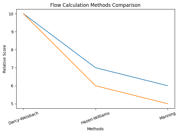
Comparison of Darcy-Weisbach, Hazen-Williams, and Manning methods based on accuracy and applicability.
Common User Mistakes
- Mixing Units: Entering pipe diameter in inches while using a formula expecting feet (common in Manning's and Hazen-Williams) leads to orders-of-magnitude errors.
- Coefficient Confusion: Using the Hazen-Williams "C" factor (roughness) interchangeably with the Darcy-Weisbach "ε" (absolute roughness) is incorrect; they are not related.
- Ignoring Flow Regime: Applying Hazen-Williams to a slow or viscous flow where the Reynolds number is low violates its assumptions and yields false results.
- Manning's "Full Flow" Assumption: Applying Manning's equation to a pressurized pipe (where it doesn't run partially full) misapplies the method.
- Forgetting Temperature Effects: Hazen-Williams does not account for viscosity changes; Darcy-Weisbach is required if water temperature varies significantly from 60°F.
Quick Formula Summary
| Method | Formula (Common Form) | Variables |
|---|---|---|
| Darcy-Weisbach | hf = f ⋅ (L/D) ⋅ (V²/2g) | hf = head loss, f = friction factor, L = length, D = diameter, V = velocity, g = gravity |
| Hazen-Williams | V = k ⋅ C ⋅ R0.63 ⋅ S0.54 | V = velocity, k = unit constant (0.849 for SI, 1.318 for US), C = roughness coeff., R = hydraulic radius, S = slope |
| Manning | V = (1.49/n) ⋅ R2/3 ⋅ S1/2 | V = velocity, n = roughness coeff., R = hydraulic radius, S = slope |
Frequently Asked Questions
What is acceptable pressure drop in a pipe system?
There is no universal single value. Acceptable pressure drop is determined by the available pressure at the source and the minimum pressure required at the furthest outlet. For water distribution, a rule of thumb is to keep friction loss below 10-15 psi (70-100 kPa) in the longest branch. For HVAC ducts, it is often expressed as a friction rate, such as 0.1 in. w.g. per 100 feet.
How do you calculate pressure drop in a pipe?
The most common method is the Darcy-Weisbach equation: ΔP = f × (L/D) × (ρv²/2). This requires calculating the fluid velocity, Reynolds number, and friction factor (f) based on pipe roughness and flow regime.
What factors affect pressure loss the most?
Fluid velocity has the most significant impact, as pressure loss increases with the square of the velocity. Pipe diameter is the next most critical, as loss is inversely proportional to the fifth power of the diameter (D5) in many empirical formulas. A small reduction in diameter exponentially increases loss.
What is the difference between head loss and pressure drop?
Pressure drop (ΔP) is a measure of energy loss in pressure units (e.g., psi, Pa). Head loss (hf) is that same energy loss expressed as the equivalent height of a column of the fluid (e.g., feet of water). They are related by ΔP = ρ * g * hf.
Does pipe diameter affect pressure drop?
Yes, profoundly. For a given flow rate, decreasing the pipe diameter forces the fluid velocity to increase. Since friction loss is proportional to velocity squared and inversely proportional to diameter, the net effect is that pressure drop is roughly inversely proportional to the fifth power of the diameter.
Why do fittings increase pressure loss?
Fittings change the direction of flow or its cross-sectional area. These changes cause flow separation, eddies, and increased turbulence. This turbulent activity dissipates fluid energy as heat, resulting in a pressure drop that is not recovered downstream.
Can pressure drop be negative?
In a passive system with no pump, pressure drop is always positive, meaning pressure decreases in the direction of flow. A negative pressure drop would imply an increase in pressure, which can only occur if there is a pump or if the pipe drops significantly in elevation, converting potential energy into pressure.
How does fluid viscosity influence pressure loss?
Viscosity is a measure of internal friction. In laminar flow, pressure drop is directly proportional to viscosity. In turbulent flow, the relationship is more complex; viscosity influences the thickness of the boundary layer and the friction factor, but pipe roughness often becomes the dominant factor.
What is the role of Reynolds number in pressure drop calculations?
The Reynolds number determines the flow regime (laminar or turbulent). This regime dictates how the friction factor is calculated. In laminar flow, friction is independent of pipe roughness. In turbulent flow, the friction factor depends on both the Reynolds number and the pipe's relative roughness.